Tutorial - Part 1

This is the first part of the QuickSR tutorial. This section provides the minimal steps required to perform symbolic regression on a synthetic dataset.

Dependencies

First of all, we need to import QuickSR and other dependencies

from quicksr import *

import numpy as np
import matplotlib.pyplot as plt

Dataset

For simplicity, we’ll use a synthetic, single-dimensional dataset, for which we already know the exact algebraic formula:

X = np.linspace(-5, 5, 25)
y = 2.5382 * np.cos(X)*X + X*X - 0.5

Here’s how the dataset looks like:

plt.figure()
plt.scatter(X, y)
plt.show()

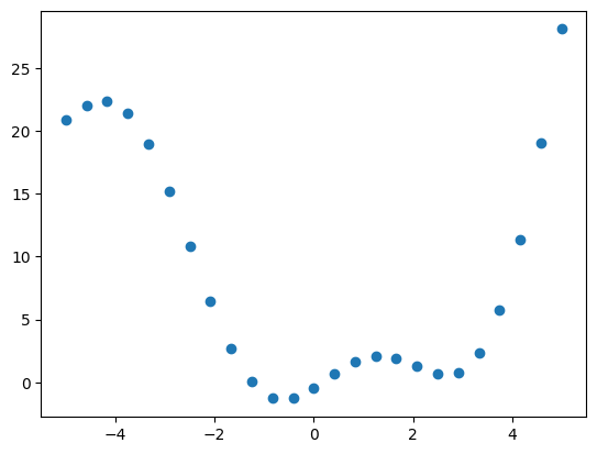
Now, our goal is to fit a curve to these 25 points. If we are lucky, we expect to find exact the expression that we have used to generate the dataset.

Configuration

Let’s start by defining the constants and “hyperparameters” of symbolic regression. First, the constant NVARS denotes the number of features present in our dataset. Since we only have a single feature (the x-axis values), we set NVARS to one.

NVARS = 1

An important hyperparameter we need to determine is the population size. This is the number of candidate expressions that will exist at every generation. For now, let’s set it to an arbitrary value.

NPOPULATION = 11200

QuickSR partitions the population into equal-size groups called islands. Each island is assigned to its own CPU core. The associated GPU kernels are also executed on the island’s own stream. Therefore, it is reasonable to set the number of islands to the maximum level of task parallelism supported by the machine. Since this notebook was executed on a 28-core CPU, we use 28 here. You can adjust this value according to your own environment. With this choice, we have 11200 / 28 = 400 expressions per island.

NISLANDS = 28

In QuickSR we have two types of constants in candidate expressions:

1. Regular constants

2. Trainable constants (also referred to as trainable weights or trainable parameters)

Regular constants arise naturally from algebraic operations. For example, the constant \(2\) can arise from the simplification of the expression \((x + x) / x\).

Trainable constants, on the other hand, are explicitly inserted into candidate expressions. Initially, these have random values. Before an expression is evaluated for loss, these constants are learned using gradient descent and backpropagation. For example, the constants \(w_{0}\) and \(w_{1}\) in the expression \(w_{0} + x \times w_{1}\) are trainable constants.

To determine the maximum number of distinct trainable constants, we use NWEIGHTS. For now, let’s set it to two.

NWEIGHTS = 2

The Model

In this step, we create a symbolic regression model using the aforemention configuration parameters. In addition, we limit the depth of candidate expressions in the initial population to one, meaning that the initial population can only consists of variables (which is just the single feature x) and constants (e.g., 2.3). Anything else will be generated during later genetic operations.

It is important to note that we can actually configure a lot more things here, but we will continue with the default choices in this tutorial.

model = SymbolicRegressionModel(NVARS, NWEIGHTS, NPOPULATION, NISLANDS,
    initialization=GrowInitialization(init_depth=1))

Training

It is finally the time to train the model and see what expression it suggests. However, before continuing, we need to determine two more hyperparameters.

1. ngenerations

2. nsupergenerations

In QuickSR, every island evolves in isolation from other islands for \(ngenerations\) many iterations. At the end of the isolation step, the best solution found by \(island_{(i)}\) replaces the worst solution found by \(island_{(i+1)}\), which is called the migration step. The entirety of this two-step process is repeated for \(nsupergenerations\) times. Thus, the total number of iterations is given by \(ngenerations \times nsupergenerations\).

Let’s set ngenerations to 5 and nsupergenerations to 4, yielding a total of 20 iterations. We will also use 500 epochs in gradient descent to fit the trainable constants. This can take some time.

solution, _, _ = model.fit(X, y, ngenerations=5, nsupergenerations=4, nepochs=500)

Island 12 Best solution: (x0) * ((x0) + (w0=-0.937014)) Loss: 13.4559
Island 0 Best solution: ((x0) - (w1=0.931526)) * (x0) Loss: 13.4561
Island 27 Best solution: ((x0) + (cos(x0))) * ((w0=-0.531155) + (x0)) Loss: 5.33177
Island 21 Best solution: ((x0) + (w1=-0.936625)) * (x0) Loss: 13.4559
Island 8 Best solution: ((w0=-0.934931) + (x0)) * (x0) Loss: 13.4559
Island 7 Best solution: (x0) * ((x0) + (w1=-0.936529)) Loss: 13.4559
Island 14 Best solution: (sin(x0)) + (((x0) + (w0=-0.861429)) * (x0)) Loss: 14.547
Island 4 Best solution: ((x0) * (x0)) - (x0) Loss: 13.4921
Island 16 Best solution: ((x0) * (x0)) - (((x0) - (w0=-0.124843)) + (w1=0.520710)) Loss: 13.2633
Island 2 Best solution: ((x0) + (w0=-0.935558)) * (x0) Loss: 13.4559
Island 18 Best solution: relu((x0) * (((x0) - (w0=0.888435)) - (w1=0.056183))) Loss: 13.4309
Island 13 Best solution: ((x0) - (w0=0.925074)) * (x0) Loss: 13.4571
Island 3 Best solution: (x0) * ((relu((x0) + (x0))) + (w0=-4.781519)) Loss: 11.2703
Island 22 Best solution: ((w0=-0.933644) + (x0)) * (x0) Loss: 13.456
Island 9 Best solution: ((x0) * (x0)) - (((x0) * (cos(x0))) / (w1=-0.393980)) Loss: 0.25
Island 10 Best solution: ((x0) * (x0)) - (x0) Loss: 13.4921
Island 5 Best solution: (w1=-2.514902) * ((x0) * (((x0) / (w1=-2.514902)) - (cos(x0)))) Loss: 0.25178
Island 26 Best solution: ((w1=-0.970122) * (x0)) * ((w0=0.949610) - (x0)) Loss: 13.319
Island 1 Best solution: ((w0=0.965956) - (x0)) * ((x0) * (w1=-0.969196)) Loss: 13.3167
Island 11 Best solution: (x0) * ((x0) + (w0=-0.936588)) Loss: 13.4559
Island 6 Best solution: ((x0) - (w0=0.937380)) * (x0) Loss: 13.4559
Island 20 Best solution: ((sin((x0) + (w0=1.096928))) + (x0)) * ((x0) * (w0=1.096928)) Loss: 9.40935
Island 15 Best solution: (x0) * ((x0) + (w1=-0.936660)) Loss: 13.4559
Island 19 Best solution: (x0) * ((x0) - (w1=0.935518)) Loss: 13.4559
Island 24 Best solution: (x0) * ((x0) + (cos((x0) + (w1=-0.025606)))) Loss: 7.99961
Island 23 Best solution: (((cos(x0)) - (1.000000)) + (x0)) * ((w0=0.414565) + (x0)) Loss: 4.92693
Island 25 Best solution: ((x0) * (x0)) - (x0) Loss: 13.4921
Island 17 Best solution: ((cos(x0)) - ((w0=0.947905) - (x0))) * ((x0) * (w0=0.947905)) Loss: 6.23782
Global best solution: ((x0) * (x0)) - (((x0) * (cos(x0))) / (w1=-0.393980)) Loss: 0.25

Island 6 Best solution: (w1=-1.292484) * ((((((((x0) / (w1=-1.292484)) - (cos(x0))) * (w0=0.968955)) * (w1=-1.292484)) / (w1=-1.292484)) - (cos(x0))) * (x0)) Loss: 0.110965
Island 8 Best solution: ((x0) + (w0=-0.531084)) * ((cos(x0)) + (x0)) Loss: 5.33177
Island 11 Best solution: (x0) * ((x0) + (w0=-0.936556)) Loss: 13.4559
Island 3 Best solution: relu((x0) * (((cos(x0)) + (w1=0.355787)) + (((w0=-0.559416) + (cos(x0))) + (x0)))) Loss: 0.908509
Island 19 Best solution: (x0) * ((x0) - (w1=0.936699)) Loss: 13.4559
Island 12 Best solution: (x0) * ((x0) + (sin((x0) - (w1=-1.530380)))) Loss: 8.00058
Island 22 Best solution: (x0) * ((x0) + (cos(x0))) Loss: 8.0091
Island 16 Best solution: (x0) * ((x0) + ((cos(x0)) * (w0=2.468650))) Loss: 0.265863
Island 24 Best solution: ((((cos(x0)) - (cos((x0) + (x0)))) + (x0)) + ((cos(x0)) - (1.000000))) * ((w0=0.407831) + (x0)) Loss: 2.84369
Island 9 Best solution: ((x0) * ((w1=0.969165) * (x0))) - ((w0=-2.528324) * ((cos(x0)) * (x0))) Loss: 0.111133
Island 14 Best solution: (x0) * (((x0) + (cos(x0))) - (w0=0.570696)) Loss: 5.10008
Island 23 Best solution: (((cos(x0)) / (w0=0.381831)) + (x0)) * ((w1=0.969165) * (x0)) Island 21 Best solution: relu(((cos(x0)) + ((x0) + (w1=-0.571935))) * (x0)) Loss: 5.10016
Loss: 0.110814
Island 5 Best solution: (w1=-1.283511) * ((x0) * ((((x0) / (w0=-1.325603)) - (cos(x0))) - (cos(x0)))) Loss: 0.113661
Island 7 Best solution: (((x0) - (w1=0.043964)) + (cos(x0))) * ((x0) - (w0=0.488436)) Loss: 5.32922
Island 0 Best solution: ((sin((x0) + (w1=1.492645))) * (x0)) + (((x0) + (w0=-0.190505)) * ((x0) + (cos(x0)))) Loss: 0.881243
Island 17 Best solution: (((w0=2.179224) * (cos(x0))) + (x0)) * (x0) Loss: 0.672588
Island 1 Best solution: (((x0) + (cos(x0))) + (cos(x0))) * ((w1=-0.150720) + (x0)) Loss: 0.957409
Island 4 Best solution: (x0) * ((x0) + (cos(x0))) Loss: 8.0091
Island 2 Best solution: (((x0) - ((cos(x0)) * (w0=-1.044665))) * (x0)) - (x0) Loss: 6.641
Island 13 Best solution: (x0) * ((x0) + (cos(x0))) Loss: 8.0091
Island 27 Best solution: ((cos(x0)) + ((w0=0.188107) + ((cos(x0)) + ((w1=-0.581908) + (x0))))) * ((x0) + (w0=0.188107)) Loss: 0.786014
Island 26 Best solution: ((x0) * (x0)) + ((w1=2.522222) * ((cos(x0)) * (x0))) Loss: 0.250837
Island 15 Best solution: (((w1=-0.546676) + (x0)) * ((cos(x0)) + (x0))) + (w1=-0.546676) Loss: 4.98454
Island 25 Best solution: (((cos(x0)) + (x0)) + (cos(x0))) * (x0) Loss: 1.19989
Island 18 Best solution: ((cos((x0) + (0.000000))) - (((cos((w0=0.998434) * (x0))) * (w1=-1.420815)) - (x0))) * (x0) Loss: 0.294657
Island 20 Best solution: ((sin((x0) + (w0=1.518123))) + (x0)) * ((x0) + (w1=-0.535243)) Loss: 5.30697
Island 10 Best solution: ((x0) * (x0)) - (((cos(x0)) * (x0)) / (w1=-0.393980)) Loss: 0.25
Global best solution: (((cos(x0)) / (w0=0.381831)) + (x0)) * ((w1=0.969165) * (x0)) Loss: 0.110814

Island 1 Best solution: ((cos(x0)) + ((cos(x0)) + ((cos(x0)) + (x0)))) * ((x0) + ((relu((w0=0.273044) - (cos(x0)))) * (w0=0.273044))) Loss: 0.257732
Island 24 Best solution: ((w1=0.969165) * (x0)) * (((cos(x0)) / (w0=0.381831)) + (x0)) Loss: 0.110814
Island 22 Best solution: ((cos(x0)) + ((x0) + (w0=-0.569545))) * (x0) Loss: 5.10003
Island 4 Best solution: (((x0) + ((cos(cos(x0))) + (cos(x0)))) + ((w1=-1.018193) + (cos(x0)))) * (x0) Loss: 0.434603
Island 12 Best solution: ((x0) + (sin((w0=1.013358) + (x0)))) * ((cos((w0=1.013358) * (x0))) + (x0)) Loss: 3.79948
Island 13 Best solution: (x0) * (((x0) + (cos(x0))) - (w0=0.568583)) Loss: 5.10001
Island 15 Best solution: ((((cos(x0)) + ((w0=0.986419) * (((x0) * (w0=0.986419)) + (cos(x0))))) + (w1=0.791313)) - (1.000000)) * (x0) Loss: 0.737316
Island 8 Best solution: ((w1=-0.199862) + (((cos(x0)) + (x0)) + (cos(x0)))) * (x0) Loss: 0.843763
Island 9 Best solution: ((x0) * ((w1=0.969165) * (x0))) - ((w0=-2.536289) * ((cos(x0)) * (x0))) Loss: 0.110826
Island 25 Best solution: (x0) * (((cos(x0)) * (w1=2.537668)) + (x0)) Loss: 0.250001
Island 20 Best solution: (x0) * (((sin((x0) + (w0=1.523799))) + (x0)) + ((cos(x0)) * (w0=1.523799))) Loss: 0.233082
Island 11 Best solution: ((((x0) * (x0)) - (w0=0.272751)) - (w0=0.272751)) - (((cos(x0)) * (x0)) / (w1=-0.393980)) Loss: 0.00207048
Island 17 Best solution: (((x0) + ((cos(x0)) * (w0=2.613319))) * (w1=0.969447)) * (x0) Loss: 0.110898
Island 19 Best solution: (((w0=-0.030835) * (x0)) - (((cos(x0)) * (w1=-2.406373)) - (x0))) * (x0) Loss: 0.167803
Island 21 Best solution: relu(((((x0) + (w1=-0.220663)) + (cos(x0))) * (w0=0.958101)) * ((x0) + (cos(x0)))) Loss: 1.46135
Island 3 Best solution: (((x0) + ((w1=-0.030438) * (cos(x0)))) + ((x0) * (w1=-0.030438))) * (((w0=2.643816) * (cos(x0))) + (x0)) Loss: 0.0922868
Island 14 Best solution: (((w0=0.393980) * (x0)) + (cos(x0))) * ((x0) / (w0=0.393980)) Loss: 0.25
Island 5 Best solution: (w1=-1.269780) * ((x0) * ((((x0) / (w0=-1.310237)) - (cos(x0))) - (cos(x0)))) Loss: 0.11082
Island 23 Best solution: (((cos(x0)) / (w0=0.381831)) + (x0)) * ((w1=0.969165) * (x0)) Loss: 0.110814
Island 26 Best solution: ((x0) * (x0)) + ((x0) * ((w1=2.538164) * (cos(x0)))) Loss: 0.25
Island 10 Best solution: ((x0) * ((x0) * (w0=0.969165))) - (((x0) * (cos(x0))) / (w1=-0.393980)) Loss: 0.110814
Island 7 Best solution: (w1=-1.288981) * ((((((((x0) / (w1=-1.288981)) - (cos(x0))) * (w0=0.969164)) * (w1=-1.288981)) / (w1=-1.288981)) - (cos(x0))) * (x0)) Loss: 0.110814
Island 18 Best solution: (w1=1.607653) * ((((sin((w1=1.607653) + (x0))) - (((x0) * (w0=0.630749)) - (x0))) * (w1=1.607653)) * (x0)) Loss: 0.065182
Island 0 Best solution: ((w0=0.121811) + (x0)) * ((((cos(x0)) + ((x0) / (w1=1.022625))) + (cos(x0))) + (cos(x0))) Loss: 0.635791
Island 27 Best solution: ((x0) * (x0)) + ((w1=2.538085) * ((cos(x0)) * (x0))) Loss: 0.25
Island 6 Best solution: (w1=-1.268650) * ((x0) * ((((x0) / (w0=-1.308976)) - (cos(x0))) - (cos(x0)))) Loss: 0.110817
Island 16 Best solution: ((x0) + ((w0=2.743777) * (cos(x0)))) * (((cos(x0)) * (w1=-0.217937)) + (x0)) Loss: 0.0977606
Island 2 Best solution: ((x0) * (w0=0.973612)) * (((cos(x0)) * (w1=1.527770)) + ((cos(x0)) + (x0))) Loss: 0.133219
Global best solution: ((((x0) * (x0)) - (w0=0.272751)) - (w0=0.272751)) - (((cos(x0)) * (x0)) / (w1=-0.393980)) Loss: 0.00207048

Island 17 Best solution: ((x0) + ((w0=2.743777) * (cos(x0)))) * (((cos(x0)) * (w1=-0.217937)) + (x0)) Loss: 0.0977606
Island 4 Best solution: ((x0) + ((w0=2.674937) * (cos(x0)))) * (((w1=-0.029810) * ((cos(x0)) + (x0))) + (((w1=-0.029810) * (cos(x0))) + (x0))) Loss: 0.0776706
Island 27 Best solution: ((x0) * (x0)) + ((x0) * ((w1=2.538164) * (cos(x0)))) Loss: 0.25
Island 16 Best solution: ((x0) + ((w0=2.761085) * (cos(x0)))) * (((cos(x0)) * (w1=-0.229538)) + (x0)) Loss: 0.0959706
Island 22 Best solution: (x0) * ((((x0) + (w0=-0.197687)) + (cos(x0))) + (cos(x0))) Loss: 0.843758
Island 20 Best solution: (((w0=-0.030835) * (x0)) - (((cos(x0)) * (w1=-2.406373)) - (x0))) * (x0) Loss: 0.167803
Island 8 Best solution: ((((((x0) / (w1=-1.288978)) - (cos(x0))) * (w0=0.969164)) - (cos(x0))) * (x0)) * (w1=-1.288978) Loss: 0.110814
Island 5 Best solution: (w1=-1.269134) * ((x0) * ((((x0) / (w0=-1.309516)) - (cos(x0))) - (cos(x0)))) Loss: 0.110814
Island 12 Best solution: (((((((x0) * (x0)) - (w0=-0.166747)) - (w0=-0.166747)) - (((cos(x0)) * (x0)) / (w1=-0.787959))) - (w0=-0.166747)) - (1.000000)) - (((cos(x0)) * (x0)) / (w1=-0.787959)) Loss: 5.89404e-08
Island 10 Best solution: (((x0) * (w0=0.969165)) * (x0)) - (((x0) * (cos(x0))) / (w1=-0.393980)) Loss: 0.110814
Island 19 Best solution: (w1=1.607653) * ((((sin((w1=1.607653) + (x0))) - (((x0) * (w0=0.630749)) - (x0))) * (w1=1.607653)) * (x0)) Loss: 0.065182
Island 1 Best solution: ((cos(x0)) + ((cos(x0)) + ((x0) + (cos(x0))))) * (((w0=-0.347165) * (cos(x0))) + (x0)) Loss: 0.184038
Island 18 Best solution: (w1=1.607655) * (((w1=1.607655) * ((sin((w1=1.607655) + (x0))) - (((w0=0.630750) * (x0)) - (x0)))) * (x0)) Loss: 0.0651819
Island 6 Best solution: (((((x0) / (w1=-1.309488)) - (cos(x0))) - (cos(x0))) * (x0)) * (w0=-1.269109) Loss: 0.110814
Island 9 Best solution: (((x0) * (x0)) + (w0=-0.394758)) - (((x0) * (cos(x0))) / (w0=-0.394758)) Loss: 0.0111579
Island 24 Best solution: ((x0) + ((cos(x0)) / (w0=0.381831))) * ((x0) * (w1=0.969165)) Loss: 0.110814
Island 7 Best solution: (w1=-1.268650) * ((x0) * ((((x0) / (w0=-1.308976)) - (cos(x0))) - (cos(x0)))) Loss: 0.110817
Island 25 Best solution: ((w1=0.969165) * (x0)) * (((cos(x0)) / (w0=0.381831)) + (x0)) Loss: 0.110814
Island 23 Best solution: (((cos(x0)) / (w0=0.381831)) + (x0)) * ((w1=0.969165) * (x0)) Loss: 0.110814
Island 11 Best solution: ((((x0) * (x0)) - (w0=0.250004)) - (w0=0.250004)) - (((x0) * (cos(x0))) / (w1=-0.393980)) Loss: 5.51772e-11
Island 0 Best solution: ((x0) * (x0)) + (((cos(x0)) * ((x0) + (w0=0.060849))) * (w1=2.531779)) Loss: 0.234816
Island 14 Best solution: ((x0) / (w0=0.393980)) * (((x0) * (w1=0.381832)) + (cos(x0))) Loss: 0.110814
Island 26 Best solution: (x0) * ((x0) + ((cos(x0)) * (w1=2.538108))) Loss: 0.25
Island 3 Best solution: (((x0) + ((w1=-0.030854) * (cos(x0)))) + ((x0) * (w1=-0.030854))) * (((w0=2.651284) * (cos(x0))) + (x0)) Loss: 0.0921245
Island 15 Best solution: ((x0) / (w0=0.393980)) * ((cos(x0)) + ((x0) * (w1=0.381832))) Loss: 0.110814
Island 21 Best solution: (x0) * ((((x0) + ((w1=-0.038990) * (x0))) + (sin((w0=1.623254) + (x0)))) + ((cos(x0)) * (w0=1.623254))) Loss: 0.100114
Island 13 Best solution: (x0) * ((x0) + ((cos(x0)) + ((w1=0.170471) + ((cos(x0)) + (cos(x0)))))) Loss: 0.687144
Island 2 Best solution: ((w0=0.969291) * (x0)) * (((cos(x0)) * (w1=2.616432)) + (x0)) Loss: 0.110831
Global best solution: ((((x0) * (x0)) - (w0=0.250004)) - (w0=0.250004)) - (((x0) * (cos(x0))) / (w1=-0.393980)) Loss: 5.51772e-11

Inference

It’s time to print the best solution.

solution

((((x0) * (x0)) - (w0=0.250004)) - (w0=0.250004)) - (((x0) * (cos(x0))) / (w1=-0.393980))

We can also display what the model prediction looks like, and compare it with the original dataset

y_original = y
y_predicted = model.predict(X)

plt.figure()
plt.scatter(X, y_original, label='Original Dataset')
plt.plot(X, y_predicted, label='Model Prediction')
plt.legend()
plt.show()

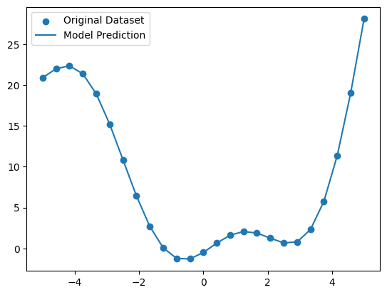
We have obtained a nearly perfect fit. It has also discovered the terms \(x*x\) and \(x*cos(x)\) in the original expression that was used to generate the dataset.